Thursday, November 12, 2020

The Case Against Using the CAPE Ratio for Relative Valuation Across Markets

Bloomberg has an article You May Regret Staying Parked in U.S. Stocks which made the case that there’s "widespread agreement" and "the answer isn’t in dispute" that foreign stocks will outperform going forward. 

Simplified version of my view of that statement.... c'mon now. Extended version of my view of that statement is in line with what Jamie Powell outlines here:

So really, it’s hard to argue that US equities are any more expensive than their European counterparts. Sure, the States might have far more stocks at trading at rich prices, but that’s by virtue of its sectoral composition, rather than it being a uniquely American phenomenon. 

But the point of this post isn't to get into the relative fundamentals of US vs foreign stocks, but rather to outline how the author made a basic error with his choice of valuation metric.


Cyclically Adjusted Price to Earnings Can Not Be Used to Compare Two Very Different Markets

The Bloomberg article states clearly that U.S. fundamentals have been superior over the last decade, which in their view is unlikely to repeat.

The jaw-dropping earnings growth generated by U.S. companies in recent years — and which propelled U.S. stocks past foreign markets during the last decade — is unlikely to return anytime soon.

Fair... but then the author uses the cyclically adjusted price-to-earnings ratio ("CAPE"), which averages the real EPS from the last decade, for the denominator in the price multiple used to compare markets.


So what's the problem with the CAPE across markets? 

The problem is the U.S. has experienced "jaw dropping" growth in EPS, while foreign stocks have not.

To the numbers... the chart below shows what the CAPE ratio would be for any given market assuming a constant trailing P/E over time (i.e. if a market traded at 10x, 15x, or 20x and it continued to trade at that exact multiple for the entire time frame). The only thing that changes in the below is the EPS growth from year 1 to year 10. Note I ignore inflation in the below, so assume growth rates are real instead of nominal.


For a company with 0% EPS growth each year, it's easy... the starting and ending multiple is the CAPE ratio. But for a company with positive or negative EPS growth, the answer may be less intuitive. EPS growth makes the CAPE higher all else equal and EPS contraction makes the CAPE lower all else equal.

So... if we assume:
  • Stocks in a market with favorable sectors and growth prospects "should" trade at 20x (and do throughout) and have grown EPS at 10% / year, the CAPE is now ~30x.
  • Stocks in a market with less favorable sectors and growth prospects "should" trade at 15x (and do throughout) and have EPS that have contracted at 2.5% / year, the CAPE is now ~13x.
Let me rephrase this to be clear... in this example the trailing P/E for the favorable market was at a 33% constant premium to the less favorable market (20/15 -1), but the end CAPE ratio of the favorable market appears as a premium of more than 100% to the less favorable market.


Conclusion

CAPE normalizes earnings when those earnings are cyclical. If your view is technology stock earnings are at a cyclical peak and industrial / banking earnings are at a cyclical trough then foreign AND US value stocks look cheap. If not, they very well may not be. 

That's your bet.

Your bet is not that valuations are remotely as extreme the CAPE implies... and there's no disputing that. 


Tuesday, August 27, 2019

Mind the Gap? Rethinking the Investor Gap Equation

Morningstar released the latest version of Mind the Gap, an annual piece which shares with its readers analysis that "measures the costs of bad timing".

In this post I'll attempt to clearly explain the math behind the investor gap calculation, share a few examples of how flows impact the investor gap, and outline why I believe these flows (thus investor gap) have little (to no) relation to investor behavior.

The result of this analysis is potential good news for investors with implications for how money is managed as 1) advisors who market their value add as "fixing bad behavior" may be selling a fix to a smaller problem than thought and 2) this may help further explain the performance of factors that have struggled in recent years IF those factors rely on poor investor behavior as some research believes.


What is the "Investor Gap"?

Morningstar shares the calculation:

To calculate fund investor returns, we adjust the official returns by using monthly flows in and out of the fund. Thus, we calculate a rate of return gener­ated by a fund’s investors. As with an internal rate of return calculation, investor return is the constant monthly rate of return that makes the beginning assets equal to the ending assets, with all monthly cash flows accounted for.
In other words, the calculation shows "how did the average dollar in a fund do over a certain time period".

The table below walks through the internal rate of return “IRR” calculation for an investor in a fund with returns that perfectly match those of the S&P 500 for calendar years 2008-2017 with an initial $1,000,000 investment at the end of 2008 and $50,000 taken out each year (i.e. the fund had consistent outflows). I use the period ending 2017 as I want to align results with Mind the Gap analysis from 2014 (the first year published) through the end of 2017. I'll get to the period ending 2018 in a later section.

The IRR weights each years cash flow (the initial $1,000,000 put in, the $50,000 / year taken out, the final balance taken out) and calculates the constant return that would have matched the cash flows an investor would have received given those flows (i.e. it matches the same final balance with the same cash flows).

The table's far right two columns match in terms of beginning and ending balance at a constant 6.92% return (with the same $50,000 / year outflows), meaning this is the investors dollar weighted return assuming the returns of the S&P 500 and outflows in this specific period. Note in this example the investor return (i.e. the IRR) < time weighted return (also called the geometric return), which means Morningstar would bucket this as a fund with a negative investor gap for this period.


Conversely, a fund with $50,000 / year inflows in this same period would have an investor return (i.e. IRR) of 9.50%, which is greater than the time weighted return, thus this fund would now be bucketed as one with a positive investor gap for this period.


How Do Flows and Returns Impact IRR?

Taking a step back, let’s first look at the weight of each year’s return if we were calculating the arithmetic return of a fund. In this case, each of the 10 years would have an equal 10% impact. In this example, the arithmetric return of the S&P 500 over the ten years ending 2017 would be 10.39% (the simple average return for each year in this period).

But flows and returns impact the return an investor receives relative to the arithmetic return (note the arithmetic return is always at least as large as time weighted return given the old +50% / down 50% = 0% average return, but a -25% return in $$ terms ($1 x 1.5 x 0.5 = $0.75).

In the next example we show the weight of each year’s return over this same 10-year period, but now assuming the weights are impacted by S&P 500 returns even with no flows (this is as simple as taking each years ending asset level and weighting them relative to one another while capping all 10 years at 100%). The shift each year is driven by the performance of the S&P 500... you can see the drop off from 2008 to 2009 due to the 37% decline and the subsequent higher balance as the S&P 500 rallied back to new highs in later years.


Now we'll look at how the above weights change in this 10-year period assuming $50,000 in inflows or outflows each year. Given the material sell-off early in this 2008-2017 time frame, an investor with outflows has a much higher exposure to the 2008 sell-off than an investor with inflows given flows and returns. 


The -37% market return in 2008 had an outsized negative impact to IRR for US equity funds with outflows (a headwind to investor returns) and an outsized positive impact to IRR for US equity funds with inflows (a tailwind to investor returns) during the 2008-2017 period. Given the path of returns within fixed income, the opposite was true for this period as absolute returns from 2008-2013 were higher than returns from 2013-2017. Below is a table summarizing the impacts to US equities and fixed income in more detail where "bad" = a headwind to investor returns and "good" = a tailwind to investor returns.

Recent drivers of flows 

Any dollar vs time weighted return analysis relies on the view that flows are driven mostly by investor behavior. My view is investor behavior ranks materially below each of the following in terms of aggregate impact:
  • Rebalancing: as stocks appreciate, investors sell stocks (selling stocks had a negative impact on investor gap in this window) to rebalance to bonds (buying bonds had a negative impact on investor gap in this window)
  • Demographics / cash demands: investors may sell stocks (selling stocks had a negative impact on investor gap in this window) to derisk into bonds (buying bonds had a negative impact on investor gap in this window), while most investors also make ongoing deposits on the way in and outflows on the way out. Given the age of the US population, Federal data shows households have been net sellers of equities for decades (selling stocks had a negative impact on investor gap in this window and older demographics were more likely to hold higher fee mutual funds).
  • Shift to passive / ETFs: this causes outflows in active (selling stocks had a negative impact on investor gap in this window) and inflows to passive (buying stocks had a positive impact on investor gap in this window). 
  • Shift to AUM advisors: this shifts investors from various higher fee share classes (selling stocks had a negative impact on investor gap in this window) to low fee (buying stocks had a positive impact on investor gap in this window)
The chart below shows the cumulative flows in US equities and taxable bond mutual funds by active and passive... we can see there were materially positive flows in every area except active US equities and US equities mutual funds as a whole (the combined flows of active and passive).

Summary:
  • Returns and flows narrowed the investor gap in the 2008-2017 period for passive equity mutual funds 
  • Returns + flows widened the investor gap in the 2008-2017 period for active equity mutual funds, active fixed income, and passive fixed income 

Real Life Example: The Case of the PIMCO Income Fund

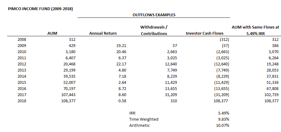
The PIMCO Income Fund is a good example of this flaw in the investor gap calculation given it has been one of the top performing bond funds over the past decade, outperforming its aggregate bond index every single year from 2009-2018. This means an investor that allocated to the fund relative to an allocation to its core aggregate bond benchmark would have benefited if they made an allocation 1) in any year in this period, while holding for 2) any time frame in this period. Flows to this fund also happened to be positive EVERY single year from 2009-2018.


Yet this strong relative performance and timing translated to a HUGE negative investor gap given the absolute performance from 2009-2013 for the fund was larger than 2014-2018 (the latter period was overweight in the IRR calculation given the strong flows). Thus, despite the fund outperforming for EVERY single investor in dollar terms relative to its index, the investor gap was more than -4% / year. The table below uses the fund's real starting AUM and annual flows and gets to an investor gap result that is pretty close to reality.


10-Year Period Ending 2018: Did Investor Behavior Really Improve?

Given the investor gap calculation had been weighed down by the return during the global financial crisis since Morningstar started putting together their Mind the Gap analysis in 2014, I have been anticipating the results for the period ending December 2018 given 2008 would roll off of the 10 year calculation. The table below shows that outflows for this period would now actually help the IRR calculation relative to time weighted returns given the lower return of US equities in more recent years in this more current 10 year window.


And here is an updated high level table outlining the expected impact.


Given these expected results would seemingly invert many of the takeaways from the previous Morningstar reports (low fee, indexing, etc... investors had smaller investor gaps for a number of potential behavior reasons), I was interested to see how an investor gap that flipped for US equities would be evaluated.

But a change in methodology of the calculation kicked that can a few years down the road given the analysis no longer looks at ten-year periods, but instead looks at the ten-year periods ending the previous 5 years. This effectively weights the studies ending 2014, 2015, 2016, and 2017 (i.e. periods positively impacted by flows) at 80% and the new period ending 2018 (that now favors outflows) at 20%.

Jeff Ptak (a great follow on Twitter not only for his investment takes, but also his music takes... and co-host of The Long View podcast) has been especially generous with his time responding to my questions over the years, as well as the change in methodology. He was gracious enough to share what the results would have been under the old methodology for the period ending 2018.

The following chart shows the investor gap by fee quintile for each of the 10 years ending 2014-2018 (the periods averaged for the new official investor gap measure) for US equities. Here we can clearly see the narrowing of the gap for all quintiles as the global financial crisis has rolled off 2018 figures, as well as the sharp reversal in terms of which investors have performed better on a dollar weighted basis by fee quintile (higher fee funds actually exhibited a positive investor gap as the analysis outlined above had expected).


The question becomes... which time frames are right? Or (in my opinion), are any of the time frames right?

My take is 1) investors clearly haven’t suddenly (year over year) gone from bad behavior to good behavior, 2) if the investor gap can be positively correlated to poor behavior at certain times and negatively correlated to poor behavior at other times, then it should probably not be viewed as something besides noise, and 3) perhaps investor behavior has improved over time and we just haven't properly measured it (investors moving from high fee to low fee, shifting towards target dates funds / robos, rebalancing as stocks have moved higher, etc... all qualitatively point the right direction).

IF we have been overstating the poor behavior of investors and/or missed their improvement, this seemingly has material implications to the scale of the value proposition advisors often use to justify exorbitant advisory fees (i.e. the need for investors to have their hands held by advisors on a continuous basis). In addition, if certain investment factors have historically relied on poor investor behavior (in the aggregate) to outperform, perhaps improved investment behavior has contributed to what has been one of the more challenging time frames for these factors in history.

Tuesday, May 7, 2019

F@ck Everything... We’re Going 120/80

Jeremy had spent most nights over the previous 30+ years on this earth in search of the next big ETF. After all, you don’t “aspire to be at the forefront of innovative ways for marrying the benefits of the exchange-traded fund structure with goals that are associated with active managers” by sitting around and doing nothing.

The problem was for as much as he searched and probed, the same tired investment ideas presented themselves over and over again. Sometimes these offerings had catchy names. Other times they had ever reduced costs. But nothing brought Jeremy the joy that he was in search of.

Disgruntled and lonely, Jeremy needed a break from the madness. So on the fateful morning of November 18th, 2017, Jeremy logged into Twitter. And shortly thereafter, his life would never be the same.


Making the Impossible, Possible

Based upon the now infamous interview with investment guru Corey Hoffstein in Barrons, the two users not so affectionately referred to as “trolls” that “lacked social skills” did what they did best.

Jake and Unrelated Nonsense argued. And argue they did.

But this argument was not like their previous arguments involving taxes or fast food. Rather, this argument was the FinTwit version of catching lightning in a bottle. You see… these two debated the merits of Corey’s idea of leveraged beta exposure by coming up with a 90% stock / 60% bond strategy that historically outperformed a 100% stock allocation with similar risk.


But that’s not where things ended.

This strategy also offered the flexibility to be held at a 2/3 weight, matching exposure of a traditional 60/40 portfolio and allowing the remaining 1/3 to be allocated to alpha strategies (click here for an older post outlining how a levered portfolio can make room for an alpha generating allocation).


Better Act Fast 

“I remember thinking this idea was just sitting there for the taking”, Jeremy is rumored to have remarked to his team back at Wisdomtree. “These idiots were just giving away their ideas for free. I had to act fast.”

And fast he acted. On August 2nd, 2018, less than one year from that fateful morning on Twitter, the ETF $NTSX was launched. Seven months later this ETF would be known as the award winning ETF, taking home the gold for best new allocation ETF.


More Free Advice

If you think this is where the story ends, you would be wrong.

On May 6th, 2019, nine years to the day of the Flash Crash, investment legend Corey Hoffstein came out with a post outlining his tactical approach to the 90/60 concept, improving outcomes for investors further (side note I do highly recommend you check it out). This was followed the very next day by the another approach I am about to share.

You see, an investor need not just use plain vanilla S&P 500 beta for the equity exposure within a 90/60 portfolio. In fact, an investor comfortable with a long-term volatility profile similar to equities could even ramp up the beta exposure past 90/60 if they could find an equity allocation that had lower volatility than the market.


Introducing the 120/80 S&P 500 Low Volatility Strategy

Since its November 1992 launch, the S&P 500 Low Volatility index has a realized volatility of 10.9%, 23% less than the S&P 500 index. As Lawrence Hamtil has pointed out in detail in a variety of posts, while there have been moments of pain, this lower volatility has not required a sacrifice in return over the longer term.


As Twitter influencer Michael Doherty pointed out, a simple allocation that swapped the S&P 500 Low Volatility Index into the 90/60 framework results in improved historical performance. The strategy now has a historical volatility a full 30% lower than the S&P 500 since 1992. As a result, an investor can keep the same 1.5 (stock):1 (bond) ratio of a 60/40 portfolio intact, but given the reduced volatility of the S&P 500 Low Volatility / Treasury portfolio can lever up the exposure 2x to 120/80 with similar historical volatility of the S&P 500.


An equity curve shows there have of course been periods this strategy would have underperformed (and past performance yada yada yada the future), but the returns have largely been consistent and outsized.


In addition, the increased exposure to equities within the strategy means that a reduced allocation to this strategy can be utilized at the portfolio level to maintain stock / bond exposure; as an example as 50% weight to 120/80 = the 60/40 traditional stock / bond notional allocation, now leaving 50% of a portfolio to pursue alpha oriented strategies.


Your move Jeremy.

Wednesday, December 19, 2018

Cash or Bonds at Low Yields and a Flat Yield Curve?

The End of an Era?

While there have been a few cyclical periods of rising rates over the past 40 years, we've largely been in one large downtrend... meaning that it has consistently paid to own bonds vs cash** or take duration risk for nearly my / many investment lives. 

Now that we've moved away from a zero interest rate policy on cash in the U.S. and the yield curve is essentially flat, this post is an attempt to pose the question of whether it still makes sense own bonds at the same scale.


The Historical Benefit of Extending Duration

Mapping the forward 10-year return of t-bills, a constant maturity 5-year Treasury bond, and a 10-year constant maturity Treasury bond against the starting yield of the 10-year Treasury, it should come as no surprise that 1) higher nominal starting yields have led to higher forward returns and given the yield curve is usually upwards sloping, that 2) longer duration bonds have generally outperformed shorter-duration bonds given their higher starting yield. 


The data in the chart above may be more easily digested when the average forward returns are "bucketed" by the starting yields of less than 4%, 4-8%, and more than 8%. Here we can more clearly see that the benefit of bonds / duration historically occurred when rates were quite elevated. 


Adjusting for a Flat Yield Curve

What the above chart does not account for is the relative starting yield of t-bills, the five year Treasury bond, and the 10 year Treasury bond. The below charts "adjust" the returns of t-bills and 5 year Treasuries to a yield equal to the starting yield of the 10 year Treasury. For example... if at T=0 t-bills yielded 1% and 10 year Treasuries yielded 3%, I added 2% / year to the t-bill ten year return. This is obviously inexact given it assumes the path of yield movements are identical in each situation despite the different yield levels.


And again... adjusted returns bucketed by starting yield of the 10 year Treasury. Now we can see the improved opportunity for cash / reducing duration; an investor can potentially (if history is a guide and this framework makes sense) reduce risk, while capturing similar (or potentially increased) return.


For those focused on tactical asset allocation, bonds are likely to outperform cash if we enter a deflationary / disinflationary environment, while cash will likely outperform if markets continue to normalize or if there are inflationary pressures. Rather than pretend to guess which situation is more likely, I would frame it as follows... are investors being fairly compensated for the increased volatility to own bonds vs cash?

With cash, you know the value will increase by the short-term rate, you just don't know what that short-term rate will be in the future. Importantly, the daily volatility of cash can be assumed to be pretty much 0% irrespective of what happens in the market. With bonds, you know roughly what that the nominal return will be, but you don't know if that return will compensate you over cash. As important, the value of bonds will fluctuate daily (historical volatility has been ~6% for 10 year Treasuries).

So, while the risk of owning bonds has likely been exaggerated for longer-term holders, there is a real increased risk of ownership relative to cash. Whether it’s the risk of less proceeds available when it comes to reallocating to other opportunities / taking withdrawals or the behavioral impact of a fluctuating account value, it’s a risk. So, if you believe the return of cash / lower duration bonds will be the same (or more) than bonds, why take that risk?


** in the above analysis I considered t-bills as a cash equivalent because they are liquid and not subject to material fluctuations in value

Wednesday, September 19, 2018

Market Timing The Credit Cycle

Over the last few years, you’ve likely heard the following competing narratives: ­

  • “Credit spreads are tight, a sign of exuberance among investors that are willing to overlook risk. This will end in tears.” 
  • “Credit spreads are tight, reflecting an environment of high economic growth and low default rates. This supports risk assets.” 
This post will outline why both of the above comments may be correct (or incorrect) by looking at asset class performance over various time frames / over recent credit cycles.


THE CYCLICALITY OF CREDIT

Corporate bond spreads can be thought of as an indicator of the overall creditworthiness of the private sector, with widening spreads either reflecting a difficult environment for companies to service their debt or the perception by investors that it may be difficult for these companies to service their debt. In this post, credit risk is defined as the difference in the option adjusted spread “OAS” (the difference in yield between a corporate bond and similar duration Treasury bond) between junk bonds and investment-grade corporate bonds, which I’ll refer to as “quality spread”.

The chart below outlines the month-end "quality spread" in percent terms going back to 1994, a time frame that goes as far back as I can get the high yield OAS data, as well as two bands reflecting one standard deviation above and below the three year month-end average spread.


Quality Spread Since 1994 (as far back as Barclays reports High Yield OAS) - %


As the chart above highlights, credit spreads can be highly cyclical, which I’ll bucket as: ­
  • Tight: More than one standard deviation below average ­
  • Normal: Within a one standard deviation band ­
  • Wide: More than one standard deviation above average 
Are tight or wide spreads a better indicator for forward risk taking? Let’s take a look.


Credit Spreads vs Longer-term Returns 

Bucketing each starting month-end period into tight, normal, or wide buckets, the forward five-year average performance of investment grade corporate bonds, high yield corporate bonds, and the S&P 500 for the 1997-2018 time frame is shown below (1997 is the first data point for the bands three years forward from the 1994 starting date).


The result is that while riskier asset classes returned more on average over the whole period: ­
  • Forward five year returns of all three asset classes were noticeably lower when the starting yield of the “quality spread” was low ­
  • In fact, both high yield bond and the S&P 500 average returns were less over the subsequent five years than the returns on the Treasury index when the starting spread was more than one standard deviation below average
  • When the “quality spread” was elevated, average excess performance was exceptionally high in both absolute and relative terms five years forward

In summary… over these longer-term windows, a low spread = a lower return (which would seem to indicate longer-term investors may currently be taking excess / uncompensated risk).


Credit Spreads vs Shorter-term Returns

Using the same 1997-2018 time frame and spread buckets, we can see that over the short-term (one-month forward time frame) the opposite narrative appears to be true: ­
  • Risk assets performed better when spreads were tight than when spreads were wide ­
  • In fact, the best short-term period for stocks were when spreads were more than one standard deviation below their average ­
  • Both high yield and stocks performed worse than Treasuries when spreads were wide 

In summary… over the shorter-term, low spread seems to = a higher return (which would seem to indicate investors may be more than fairly compensated to take risk given current fundamentals).


RISK / RETURN BY THE LEVEL AND DIRECTION OF SPREAD

The below charts break out investment grade bonds, high yield bonds, and S&P 500 further, charting the return (geometric one month forward annualized) ­and risk (standard deviation) by:
  • Spread levels (narrow, normal, or wide) ­
  • Spread direction (i.e. whether the "quality spread" has narrowed or tightened) 

Investment Grade Corporates

Geometric Annualized Forward One-Month Return vs Month-End Starting Yield / Direction of Spreads 


Investment grade corporates provided positive performance in all of the various environments in this time frame, but volatility did pick up when spreads were both elevated and widening (as a frame of reference, IG Corporate bonds did outperform Treasuries in all of these environments except when spreads were elevated and widening - a period where they underperformed by 6%).


High Yield Corporates

Geometric Annualized Forward One-Month Return vs Month-End Starting Yield / Direction of Spreads


The results for high yield seem more interesting. High yield returns were relatively steady in both low spread and “normal” spread environments, but the volatility of high yield was materially lower when spreads were narrow. Things were especially interesting at higher spread environments as there was: ­
  • Underperformance: when spreads were wide and widening (“catching a falling knife”) ­ 
  • Outperformance: when spreads were wide and narrowing (an investor was able to successfully capture these higher than normal yields in this window) 

US Stocks

Geometric Annualized Forward One-Month Return vs Month-End Starting Yield / Direction of Spreads 


S&P 500 returns were especially strong when spreads were narrow, as well as when spreads were “normal” and moving wider (perhaps noise over the previous month presented a buying opportunity). What I found interesting was the linear relationship between the level of spread and volatility (narrow spreads = much lower volatility). Finally, I found it interesting that the performance of US stocks was poor when spreads were elevated (irrespective of whether spreads were narrowing or widening, unlike the divergence in performance within high yield).


SUMMARY

The good news is the above analysis may provide some interesting signals for those with the flexibility to allocate tactically.

The bad news is that while I think the relationship between spread and the shorter-term performance outlined above makes logical sense, it may not work going forward.

So the next time someone asks for a quick answer as to whether tight spreads have been a sign of exuberance among investors who were willing to overlook risk (which will end in tears) or an environment of high economic growth and low default rates, supporting risk assets... you can now respond.

It depends.

Wednesday, June 20, 2018

CAPE of Good Hope? P/E Divergence as a Performance Signal

Lawrence Hamtil recently shared a Vanguard paper with me that was surprising given it indicated the trailing twelve month price-to-earnings ratio "TTM P/E" was nearly as strong a predictor of forward 10-year equity returns as the cyclically adjusted price-to-earnings "CAPE" ratio going back to 1926. My assumption had been that the CAPE ratio (which uses smoothed 10-year real earnings) would be the much better of the two ratios given it reflects the longer-term earnings power of companies within the index, rather than the (potentially at times) cyclical peak. 

This post will dig into:
  1. the historical relationship between the TTM P/E and CAPE ratios and forward returns
  2. the historical relationship between the TTM P/E and CAPE ratios, and how that relationship has changed in recent years
  3. how these ratios may potentially be used together to help predict shorter term market performance

Backdrop: The Surprising Predictive Power of TTM P/E

While perma-bears seem to enjoy highlighting metrics (debt, rates, growth rates, etc...) that have no predictive power for either short or long-term forward equity returns, valuations themselves have mattered. As I’ve highlighted in previous posts, higher valuations (as defined by an elevated CAPE ratio) have historically resulted in lower long-term forward returns. Vanguard replicated this result for trailing P/E, which surprised me given the backward looking / shorter-term / cyclical nature of the TTM earnings component in the denominator of the P/E ratio.

Per Vanguard:
We confirm that valuation metrics such as price/earnings ratios, or P/Es, have had an inverse or mean-reverting relationship with future stock market returns, although it has only been meaningful at long horizons and, even then, P/E ratios have “explained” only about 40% of the time variation in net-of-inflation returns. Our results are similar whether or not trailing earnings are smoothed or cyclically adjusted (as is done in Robert Shiller’s popular P/E10 ratio).
  

Given my need to replicate anything I see to personally believe, the below charts replicate this analysis with a scatter plot for each updated through May 2018 (the Vanguard piece is through 2011) using data from Shiller (the dotted line shows the ratio as of May 2018). We see both relationships remain strong, though the CAPE’s predictive power has improved quite a bit (more on that below) since 2011.


The Changing Relationship Between the CAPE and TTM P/E

The reason the CAPE shows a higher predictive power in updated results is due to the divergence of the two ratios leading up to and through the global financial crisis “GFC” when earnings collapsed, causing the TTM P/E to spike, which in turn made the US equity market seemingly more expensive as it sold off. 

Meanwhile the US equity market appeared quite cheap on a CAPE basis (it hit a ~30 year low), which turned out to be the correct signal. In the following chart we can see the close relationship between the two ratios following the Great Depression through late 1990’s, then the divergence seen first during and after the technology bubble (note the chart stops at 50 to show the data more clearly, but the TTM P/E spiked to 86 in October 2008).


The impact of this divergence is especially clear in the rolling ten year correlation of the TTM P/E and CAPE ratios.


As a result, in the more recent periods that capture the Internet Bubble and/or GFC at the back, middle, or the front of a 10 year rolling period, the CAPE has been extremely predictive (89%), while the TTM P/E has been less so


The Potential Use of the CAPE and TTM P/E to Make Allocation Decisions

The following chart shows the difference between the two ratios over time. We can see that for a ~60 year window following the Great Depression to the beginning stages of the Internet Bubble they moved together closely. We can also see the more recent divergence.


And this is where I think things get interesting and potentially less intuitive.

Historically, when the CAPE was elevated (meaning markets were potentially at risk from a valuation standpoint) and the CAPE > TTM P/E (meaning recent earnings in the TTM denominator are higher than the smoothed 10-year real earnings), forward short-term performance has been just fine. It's when the CAPE was elevated (again… meaning markets were potentially at risk from a valuation standpoint) and CAPE < TTM P/E (meaning recent earnings have lagged the smoothed 10-year real earnings) that short-term performance hasn't just been poor, but outright negative.

In fact, looking back at the chart above we can see the CAPE ratio exceeded the TTM P/E by a substantial margin before the major market corrections of the Great Depression, Internet Bubble, and GFC, but when the CAPE flipped below the TTM P/E is when each sell-off really took hold. Note that in the Great Depression the US equity market continued to sell-off even after the CAPE got to seemingly attractive levels.


My takeaway from all of this remains that forward long-term returns are likely to be low relative to history (both CAPE and TTM P/E point to that likelihood), while the shorter-term outlook looks better. Investors tactically holding US stocks may be well served by what has historically been strong equity performance in elevated valuation environments when current earnings remain strong and/or the upward trend of the market stays intact. But buyer beware... should either earnings or the positive trend of the market shift, current valuations increase the risk that this may end up viewed as a period of calm before the storm.

Wednesday, January 31, 2018

The Behavioral and Performance Benefits of Trend Following

When we tell our investors to invest for the long run, we have to make sure the short run doesn’t kill them first… Investing for the long run isn’t bad advice, it’s just unrealistic. It doesn’t take into account human behavior.

-Andrew Lo (HT: Andrew Thrasher)


Trend following has historically provided strong long-term returns with materially reduced drawdowns relative to a traditional buy and hold investment, but none of this matters if an investor cannot stick with the strategy through periods of relative underperformance. This “opportunity cost” is often felt the most during periods when more traditional allocations outperform.

The consistency of a trend following strategy’s relative performance vs a 60/40 portfolio (impacting the ability for investors to stick with trend following) is the basis of an argument that’s taken place offline (yes, I also argue offline) with a FinTwit friend who is a huge proponent of buy and hold. It’s progressed to the point that we’ve discussed making a mini (very mini) Buffett style bet related to whether trend following or a 60% US Stock / 40% Bond allocation will outperform over the next five years (with money going to the winner's charity of choice).

Given we've hit a dead-end due to his view that the result will be a coin flip (i.e. random whether trend or buy and hold outperforms, thus even if he were to lose it would be random as well), I thought I would put my case forward in this post outlining why I think trend following has a much higher probability of outperforming a 60/40 portfolio in most environments and especially in the current environment.


Backdrop: What is Trend?

As outlined in a previous post:

In a nutshell, trend following is simply a means of determining if you will own an asset based on its recent price history. 
One simple set of trend following rules are: ­
  • If the S&P 500 Total Return Index > 12-Month Moving Average, Own Stocks ­ 
  • Otherwise Own Bonds
The diagrams below depict how those without an understanding of trend following often believe it works vs how it really works. The original image on the left is used with permission from Carl Richards and outlines how poorly behaved investors often act, while my revised version on the right outlines what trend followers attempt to do (follow Carl on Twitter @behaviorgap).


Buy and hold investors seem to perceive trend followers in a similar light as these poorly behaved investors, chasing strong returns higher and selling out once markets have completely rolled over. In practice, trend following buys / sells after major turning points, thus gets back into markets once a new trend forms and holds until there is another turning point... often much later than when the investor would have otherwise preferred to sell. The opportunity cost of trend following is the willingness to miss initial turns and to be wrong over many intermediate periods until a new long-term trend emerges.


How Often Does Trend Following Outperform?

As the chart below shows, trend-following outperformance has occurred at a much higher rate than a coin flip and that beat rate has increased over longer periods. This specific 12-month trend model outperformed a 60/40 portfolio over ~80% of rolling 60-month time frames since 1926 and 90%+ of the time over 10 and 15 year periods. 


To get a better sense of when these periods of outperformance and underperformance occurred, the following chart breaks out when trend following outperformed a 60/40 portfolio (blue) and when it did not (white) over rolling 60-month time frames. 


A few things to note:
  1. the trend following model outperformed a 60/40 portfolio consistently
  2. the trend following model outperformed over extended periods of time
  3. periods of trend following underperformance were short lived and clustered
  4. periods of relative underperformance were more likely to occur when the opportunity cost associated with moving away from a 60/40 portfolio were high
Specific to point #4, the chart below shows the historical yield of a 60/40 portfolio (i.e. what can be viewed as the likely opportunity cost of trend following). We can see that a high starting yield that compressed quickly in the mid 1930's coincided with the underperformance that took place in the late 1930's / early 1940's, while the huge yield compression of a 60/40 portfolio in the mid 1980's coincided with the challenging relative performance in the late 1980's / early 1990's.


Current Expectation

Simply put, the starting yield / opportunity cost of a 60/40 portfolio is extremely low at ~3%. Historically, when we split the universe into buckets when the starting 60/40 yield was above or below the long-term 6% average (3% higher than the current level), we can see the increased likelihood a trend following strategy outperforms at lower starting yields. In fact, the historical beat rate over rolling 5 year time frames moves up to 85%.


Conclusion

I really like the way my friend Wes from Alpha Architect framed this decision:
Flip it and make trend following the benchmark and consider buy and hold. Works sometimes, doesn't work other times, but you eat massive tail risk with buy and hold, therefore isn't worth the risk/effort.
In other words, if trend following is your base allocation, would you as an investor allocate to a different strategy that underperformed at a 70%+ rate over 3-5 year rolling time frames and 90-100% of rolling 10-15 year time frames, and had materially more downside risk? Not only would I not make that allocation, I'd love to bet someone with proceeds going to charity that trend following would outperform.


Appendix: Tax Efficiency of Trend Following

A common question that comes up related to trend following is its tax efficiency. The reason I ended up ignoring the tax issue as a detriment to trend following in the analysis is that trend following may actually be more tax efficient than a buy and hold allocation that includes taxable bonds.

A few reasons:
  1. A trend following solution can be structured utilizing futures, which are taxed at 60% the long-term rate and 40% the short-term rate, making it pretty similar to a 60/40 portfolio
  2. Even with cash holdings, trend following can be tax efficient as the large gains in stocks are often held much longer than 12 months (i.e. are taxed at the long-term rate). The chart below shows the length of each past isolated trend, along with the gains earned in these trends showing that significant gains were often taken years after the initial trend signal.


Tuesday, December 5, 2017

Can Time Solve the Issue of High Valuations?

“Time solves most things. And what time can't solve, you have to solve yourself.” - Haruki Murakami 

Recent research by GMO outlined that wide profit margins, low levels of inflation, subdued economic volatility, and low 10 year treasury rates have led to high valuations for both U.S. stocks and bonds. Yet irrespective of why valuations are high relative to history, what an investor pays for a dollar of earnings or a dollar of bond coupons directly impacts the forward return they receive. This is generally understood by investors who have accepted the likelihood that returns will be low over the next five or even ten years. What has been discussed less, or often dismissed outright by buy-and-hold long-term investors, is the similar challenge investors may face over much longer periods of time given high starting valuations.


The Issue: Annualized Returns Can Mask the Effect of Compounding 

Annualized returns are commonly used to compare asset class performance over various time frames. The issue is annualized returns trivialize the effect of compounding, especially over longer periods. As an example, the following chart compares annualized returns for:
  1. an investment that is down -50% in year 1, which then returns 10% each year for the next 29 years
  2. an investment that returns 10% each year for the full 30 years 
We can see the large return gap between the two investments in year 1, as well as what appears to be a narrowing of that gap over time from a 10% annualized differential in year ten to a 3% annualized differential in year thirty. 


In reality, the return gap is getting larger in dollar terms as the same 10% earned each year after year one is from a much larger base for the investment that was not dragged down by the initial 50% decline.


A Revised Perspective

One way to view valuation of the U.S. stock market is the cyclically adjusted price to earnings “CAPE” ratio (a measure of the price an investor pays for each $1 of historical normalized earnings). This ratio can be converted to a yield by inverting it (i.e. a CAPE of 30x = 1/30x or a roughly 3% yield) as a means of making it more comparable with current bond yields. We can then calculate a yield for a traditional balanced 60% stock / 40% bond portfolio “60/40”, by using the formula ‘60% CAPE yield + 40% bond yield = 60/40 yield’.

This 60/40 yield has provided strong explanatory power for forward annualized ten year real (after inflation) returns going back to 1926 (Ibbotson data inception).


This 60/40 yield has also provided strong explanatory power for much longer 30-year forward annualized returns. The issue is annualized returns makes it appear that the range of outcomes, relative to starting valuations, narrows over longer periods of time, an argument commonly used by buy-and-hold investors. In reality, the comparison of annualized returns over different time frames masks the compounding effect of these seemingly small return differences.


The following chart removes this effect by showing the real growth of $1 for each these starting valuations over 10 and 30 years instead of annualized returns. We can clearly see that the gap in dollar terms widens significantly over longer periods, as the compounding effect has more time to work its magic.


The “we are here” line in this chart highlights how extreme current stock and bond valuations are relative to history, creating an environment where time itself may not be a solution to the valuation challenge.


 What Can an Investor Do? 

For an investor looking to improve their outcome, there are a variety of options available, including: ­
  1. Search for Value: reallocate capital to segments of the US equity market (or outside the US equity market) that may be more attractive ­
  2. Identify Alpha Opportunities: rethink the value proposition of active management, especially within less efficient areas of the market ­
  3. Follow the Trend: utilize trend following to manage equity exposure 

The first two options are familiar to most investors, but trend following may be less so. In a nutshell, trend following is simply a means of determining if you will own an asset based on its recent price history. One simple set of trend following rules are: ­
  • If the S&P 500 Total Return Index > 12-Month Moving Average, Own Stocks ­
  • Otherwise Own Bonds 

Given this simple trend following model can never result in monthly outperformance vs the S&P 500 when the market is up, as the most it can own is 100% stocks, it will underperform during most bull markets relative to the S&P 500. However, it may still outperform a 60/40 portfolio in these environments as it is not weighed down by an allocation to bonds. Conversely, the strategy will outperform the S&P 500 in down markets over time and, importantly, it has the potential to side step a major market correction that impairs the compounding effect that has historically impacted long-term returns when valuations have been elevated (more on why trend / momentum works here).

The below chart updates the 30 year real growth of $1 with returns for this basic trend following strategy, comparing the returns generated to the original 60/40 buy-and-hold portfolio over similar periods.


While there are still material differences in the historical growth of $1 depending on the starting valuation, the trend following strategy generated dollar growth that was consistently higher than that of a 60/40 strategy and produced returns that were higher even at low starting yields than that of a 60/40 portfolio at much higher starting yield levels.


Conclusion 

Buy and hold strategies work best when stocks and/or bonds are cheap. When valuations are extended and starting yields are low, an investor should look to allocate to cheaper areas of the global market, rethink the value proposition of active management, and/or be prepared to reduce stock market exposure if profit margins, inflation, volatility of GDP, or 10 year treasury rates (that pushed valuations higher) reverse course.

Tuesday, November 28, 2017

Volatility May Feel More Painful the Next Time Around

Stock and bond markets have been extraordinarily quiet since February 2016 lows. How quiet? A 60/40 portfolio consisting of the S&P 500 and the Bloomberg Barclays Aggregate Bond Index has a 12-month standard deviation of (wait for it)… 2.2% ending October 2017. This is the lowest period of volatility since the inception of the aggregate bond index back in 1976.


My own behavior has been impacted by just how boring markets have been, as I’ve slowly seen my own risk tolerance ramp up. In addition to thinking that I really need to rebalance, I’ve been thinking about the consequences of a world in which many investors haven’t experienced a material drawdown in many years / potentially in their entire investment lifetime. For those of us that are relatively young, even if we've lived through the 2000-01 dot com bust or the 2008-09 global financial crisis, it’s likely many of us haven’t experienced any material loss of wealth.


Viewing Market Volatility Through a $$ Lens

Let me explain with an example…. I graduated from college in May 2000, thus the below drawdowns are what I would have experienced in a 60/40 portfolio since I started my working career.


A well weathered investor I must be having faced two of the largest drawdowns in US history? Well... let’s take a look at this return history from a different perspective.

Rather than in percent terms, let’s look at the drawdown in dollar terms assuming an investor put $1000 in the market at time = 0 and added an incremental $1000 more than the previous year... each year (i.e. $1000 at time = 0, $2000 at T + 1, $3000 at T +3, etc…).


We can see from the above chart that the 2000-02 downturn may have seemed painful, but may as well not have existed in terms of consequence to an investor this early in their wealth accumulation (not to mention this investor was much less likely to have the stress of providing for a family). Even the 2008/09 downturn was quite minor in the grand scheme of things, matching the dollar drawdown of the tiny 5% drawdown experienced in late 2015. In addition, during the early stages of wealth accumulation, the ability for contributions to materially make up for market declines helps with the mental issue of otherwise seeing the value in your investment account fall (i.e. $10k is a huge contribution when your balance is $50k, $20k is much less so when your balance is $300k).

And where do many of us sit now?

For those of us fortunate to have accrued wealth over the last 10-20 years, we should anticipate a high likelihood of experiencing the largest dollar downturn of our lives at some point in the near future. In fact, in the scenario outlined above, a 15% drawdown from here would result in a loss ~4x larger than that experienced during the global financial crisis.

The implications to me are as follows:
  • Reevaluate your risk tolerance: not by the comfort level experienced over the past few years or even your entire investment life, but by what you should expect in the years to come given your current financial and life situations 
  • Create a game plan: for how you should / will react when market volatility “normalizes” (trend can be your friend)
  • Prepare for market volatility that doesn’t just “normalize”: but instead overshoots to the upside if / when markets do correct
We have a lot of market participants (myself included) that have never experienced any real turmoil and poor behavior always follows.